Track the past, plan the future

At this age and advancement of our society - regardless of the stage of life you are in - one of the most important aspects of life is to have a stable base, a foundation of financial stability.

To achieve this, let's build a tool together: a financial tracker and planning tool, that will have some other magical properties.

No, not that advanced that you see on the featured image, a simpler one: a spreadsheet. Yes, you heard that right, let's build a spreadsheet.

Open up Excel, or Google Sheets, or any other popular spreadsheet application. For the sake of simplicity and easiness, I'm going to use Google Sheets.

Create a new sheet. Name it "Finances 2024"

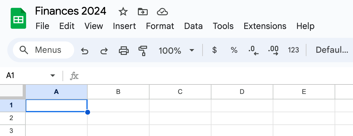
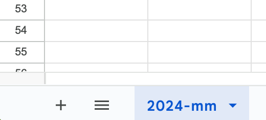
Since we are building a reusable template name the tab (at the bottom) "2024-mm", where "mm" will be replaced later with the number of the month (for example for October, it'll be 2024-10).

This tool will allow you to track your financial activities and plans on a daily basis for one month at a time. Of course, you can have as many new tabs (for each month) as you like.

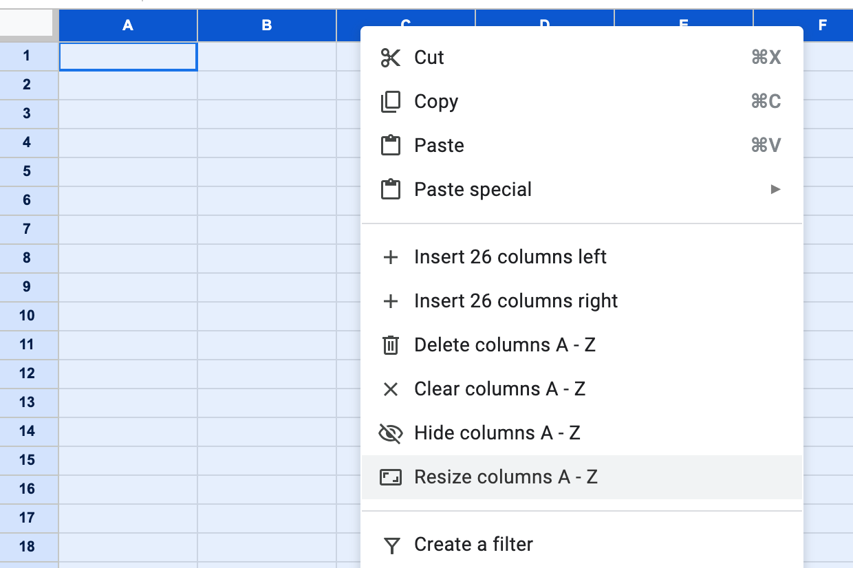
Select all the columns (by default you should have a limited number of columns, usually only 26, but we will need more), and by right clicking the header row resize all columns:

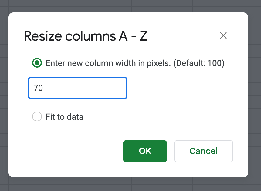
A width of "70" will do:

Good! Still with me? Let's carry on.

Next: while still all columns are selected go to the very last one (column "Z") and right click on the header row. This time select "Insert 26 columns right".

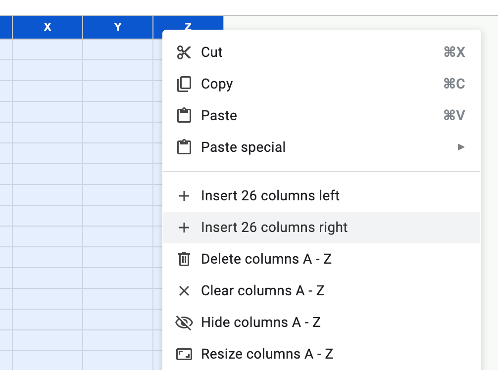
Great! We now have enough columns to work with.

We are going to have a dedicated column per day in a month. (At this moment it does not matter how many days are in a specific month, we will add 31 to this template sheet anyway and later on we will adapt).

Starting from column "D" start numbering the columns. You don't have to manually number all of them! It's enough just to number the first two, and then with a neat move we will cover the entire range.

Follow me here: add "1" to column "D", add "2" to column "E" and then select the two cells. (You should see something similar to the above screenshot.)

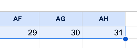
Now: left click on the blue dot - and while NOT releasing (keep holding) the mouse button - drag the selection over to the columns to the right, right until column "AH".

That's right: we have just created the numbers from 1 to 31!

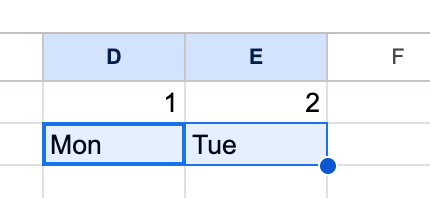
To make it more humanly consumable, we will add the names of the days too, in a similar way: go back to column "D" and add "Mon", step right and in column "E" add "Tue". Again, use the same magic here, so you don't have to do it for the entire week.

You already know the drill: while both "Mon" and "Tue" are selected, drag the blue dot to the right till column "J". There you go:

Add another small improvement - you will thank me later 😄: select "Sat" and "Sun" and apply a background colour. For my example I simply used a light grey colour.

Select all the 7 days (with the already colour-coded weekend days) and copy & paste it to the right - until you reach the 31st day.

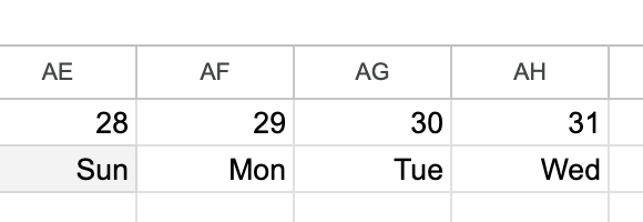
At this point you should see something like this (above) at the end of the numbered columns.

Awesome! We are getting there!

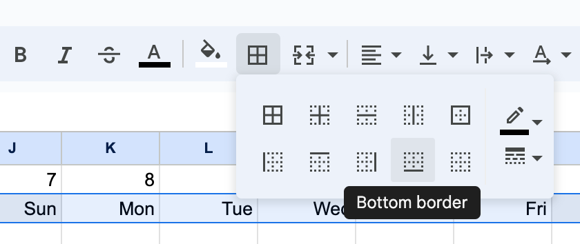
It's not mandatory, but at this stage you can draw a black line at the bottom of row "2" by selecting the entire row and then:

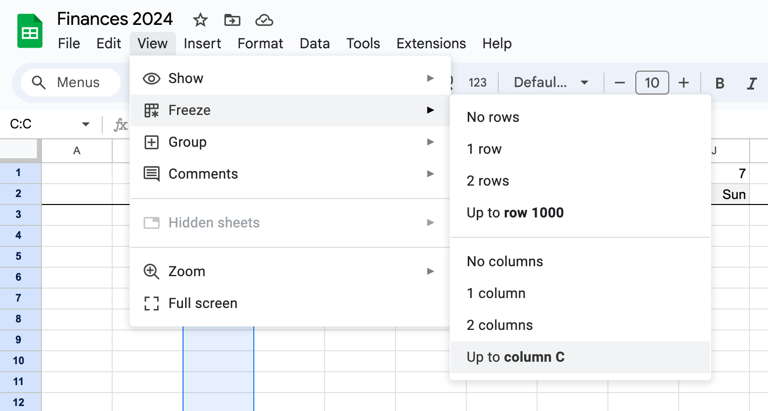
Next trick: freeze the columns up to column "C". This will became very useful later. (To manage the entire grid as the days pass and also it's useful if you are using smaller screens, like on tablets.) Simply select the entire column "C" and then:

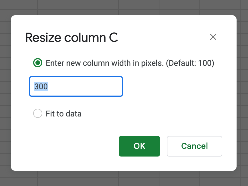
Also, while we are at it, resize column "C" to "300": we will need that extra space there soon:

Take a break here! Phew..... Almost there!

Now we will add the rows: it's so much more fun!

First, we will create the section for our income(s):

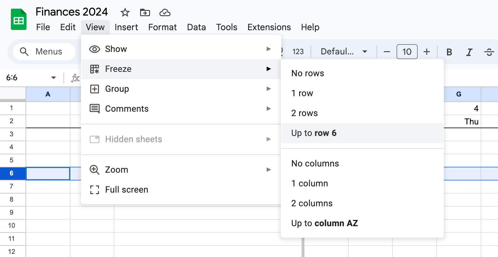
To achieve a similar "frozen" state for row six, select the entire row, and then:

Great!

Next: we will list all of our expenses - let's start with the biggest one!

Here, let me pause for a moment:

Depending on your life stage (maybe you are a student still living with your parents, maybe you manage an entire household) your expense categories (and also your income sources) may vary very much. But that's OK! A spreadsheet is super flexible, it can handle anything!

To give you and example - again, this is mostly made up - you should have something like this:

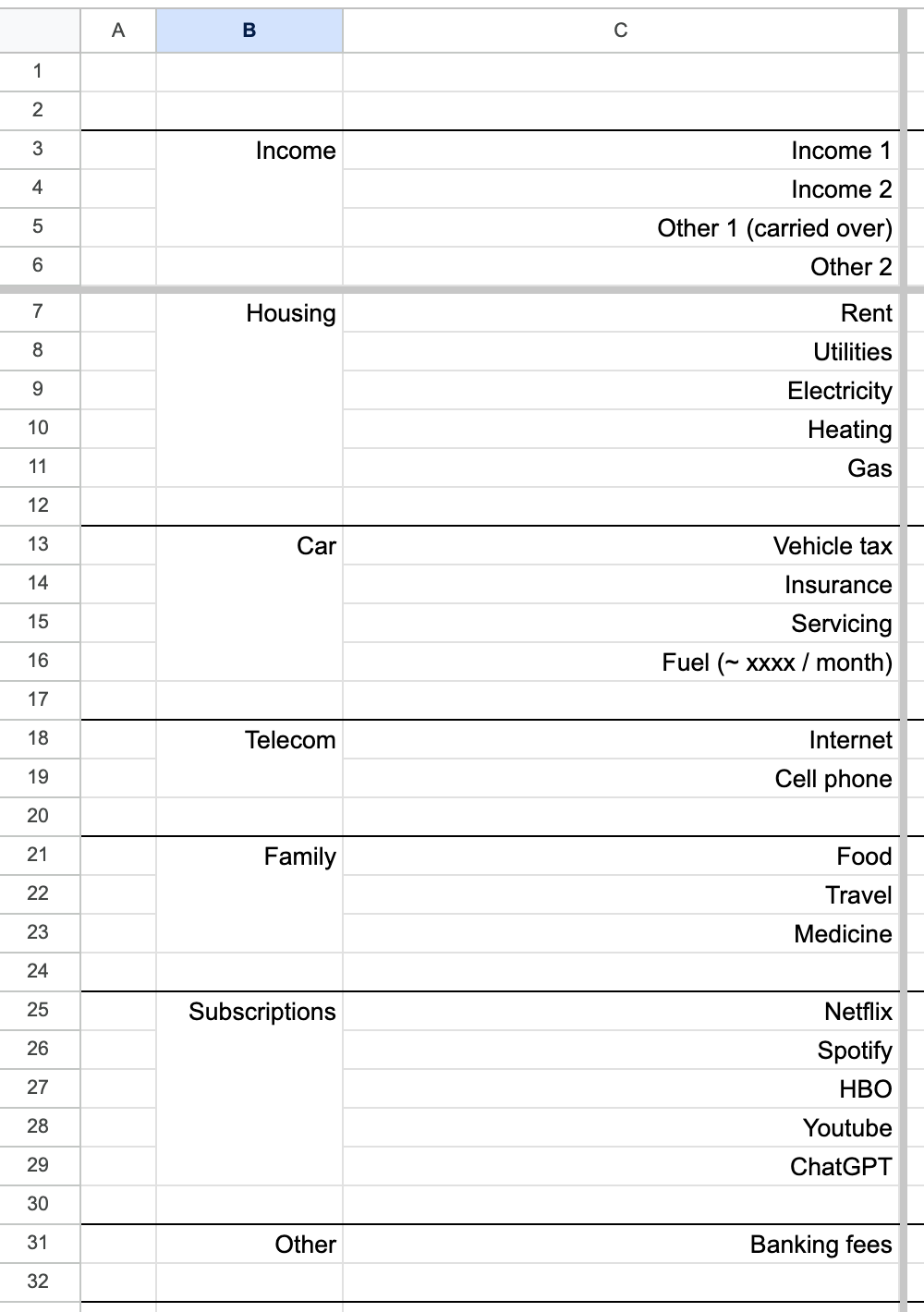
Alright! So what's the magic here? We have the days of the month in columns and the income and expense categories in rows. What's the big deal?

Well, this is just the "skeleton", a "frame" if you like. We need to apply some more magic and it will start working (like magic)! Trust me, you will like it!

Add one more section below:

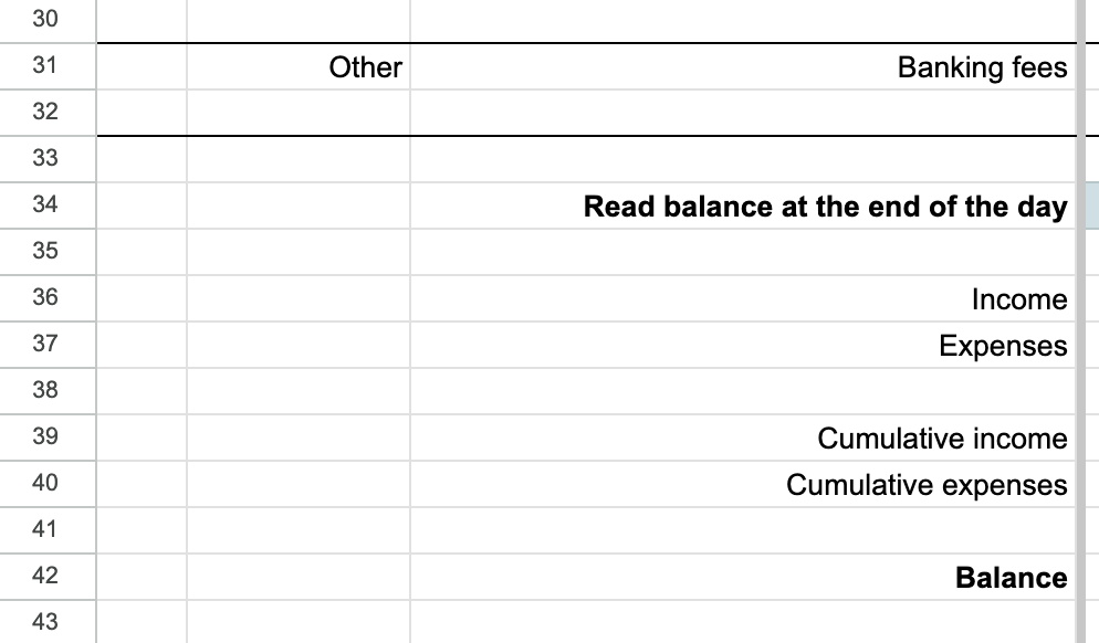
From this point, we will only add some formulas, and that's it!

I guess (hope) you already know what to do next:

• in cell "D36" add the following: =SUM(D3:D6)

What does it do? Well, it simply calculates the total value of all of your income(s) for the very first day of the month.

Not so exciting, isn't it?

With an elegant move select cell "D36" and with the blue dot apply the same formula to the entire row, up until "AH36".

Remember, the cell "D36" contains:

If you did the "blue dot move" correctly, in cell "AH36" you should see:

This sets us up for a good start: wherever you put a valid numeric value in the "income" section (rows between 3 and 6) the total daily values will be displayed in row "D36".

At this point, I guess you already know what comes next: the same process for all the expenses:

• in cell "D37" add: =SUM(D7:D32)

and repeat the process of selecting the cell ("D37") and using the blue dot drag & move till "AH37".

That's right: you now have got all of your daily expenses summed up in row 37!

We are not finished yet!

Take another break!

Back? Good.

What's left is to apply formulas to the

• Cumulative income
• Cumulative expenses, and the
• Balance rows.

On "Day 1" (in column "D") the formula is very basic:

• in "D39" simply add: =D36
• in "D40" add: =D37

BUT!

From "Day 2", things will get a bit more complex - but not by much:

Here we need to add any NEW income (or expense) to the previous day's income (or expense). Let me help you out here:

• in "E39" add: =D39+E36
• in "E40" add: =D40+E37

And only NOW you should do the magic "expansion" and "spreading" the formula across the rows:

• select "E39" and drag the blue dot all the way to "AH39"
• select "E40" and drag the blue dot all the way to "AH40"

OK, I get it, you still don't see the magic. Don't worry, it will work!

...here comes the VERY LAST BIT: add formulas to the "Balance" row.

This is very simple, because on a daily basis (for each column) we simply need to do the basic math of

• cumulative income (e.g. "D39") - cumulative expenses (e.g. "D40")

So, "D42" should look like:

From here you know the drill: blue dot at "D42", drag across till "AH42".

...AAAAANNNNDDDDD, we are done!

Now is the time where the magic begins to unfold: you can now start adding values to the grid:

• on which day do you get your salary? add it to that cell (in row 3 or 4)
• on which day(s) do you fuel your car? add those values to the right column (in row 16)

Experiment, play with it, but first, please make a copy, or "duplicate" the sheet:

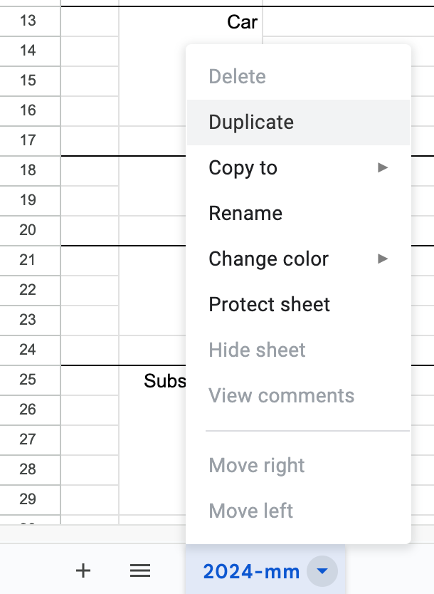
There you go, now you have your very own daily financial tracker, planner and "what-if" simulator.

Don't forget to add the income(s), expenses as time goes on, you have to do it every single day.

DONE and DONE!

Here is part 1 - covering all the steps above. Have a look: